*Originally posted for students Nov 2025.
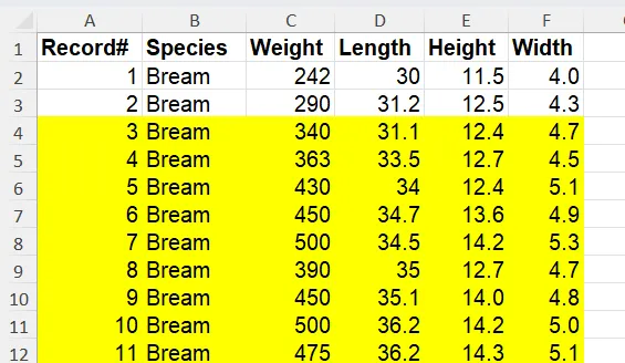
Here is a quick conditional formatting example that shows how to format individual cells vs formatting a whole row. The difference is in the Applies to area.
When you format individual cells in a column, this is what the rule looks like:
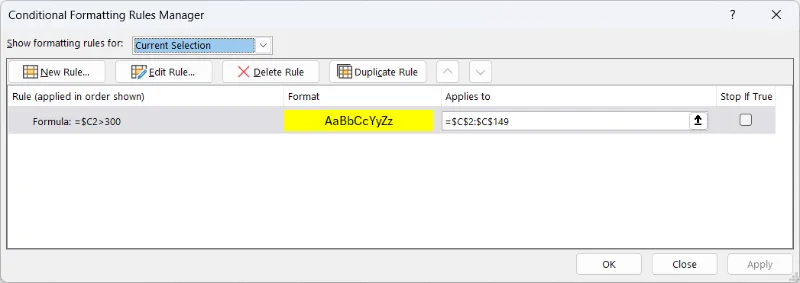
The formula is =$C2>300. This allows the row to change as we do evaluation but we stay locked on the C column.
The formula applies from $C$2:$C$149. This means that we’ll perform the formatting only on these cells in column C. Our data has headers in row 1 that we don’t want to evaluate.
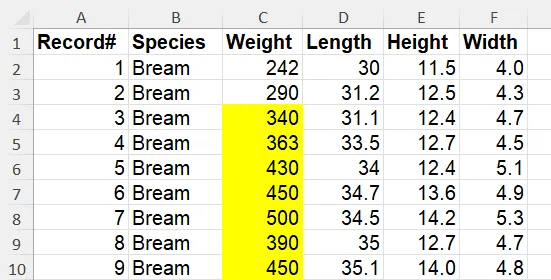
Overall what happens is that every cell from C2 down to C149 is evaluated and if that cell is greater than 300, the cell is formatted.
If we used a reference in the formula with both $ like $C$2 or $C$4 then only that individual cell would be evaluated and the entire applies to area would be formatted based on the value in that one cell. If the formula were =$C$2>300 then all cells C2:C149 would not be formatted because C2 is not greater than 300. If the formula were =$C$4>300 then all cells C2:C149 would be formatted because C4 is greater than 300.
This is the result of the rule above:
When you format a whole row, this is what the rule looks like:
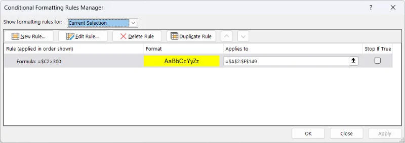
Notice that the only change in the rule is the Applies to section. This now includes the columns from A to F instead of just column C.
Overall what happens is that every cell from C2 down to C149 is evaluated and if that cell is greater than 300, the cells from columns A to F in that row are formatted.
This is the result of the rule above: